lapply-based Parallelism

3. Introduction

lapply-based parallelism may be the most intuitively familiar way to parallelize tasks in R because it extend R's prolific lapply function. It is the first class of parallelism options in R, and we will continue to use the k-means clustering example described in the introduction to parallel options for R page to demonstrate how such a task can be parallelized in a reasonably familiar way.

3.1. lapply: halfway to parallel

As with almost every form of parallel programming, you've got to take one step backwards to make two steps forwards. In a practical sense, that means making our k-means calculator a little more complicated so that parallelizing it becomes possible. The following script is functionally the same as our serial example above:

data <- read.csv('dataset.csv')

parallel.function <- function(i) {
    kmeans( data, centers=4, nstart=i )
}

results <- lapply( c(25, 25, 25, 25), FUN=parallel.function )

temp.vector <- sapply( results, function(result) { result$tot.withinss } )
result <- results[[which.min(temp.vector)]]

print(result)

Seeing as how this code is functionally equivalent to the code in the previous section, there is a lot more complexity added here that ultimately does nothing useful. I've highlighted all of the new cruft we've had to add to our code in blue, only those lines that remain uncolored resemble the code that actually does the k-means calculation in the simple, serial case.

Here are the key features of the changes:

1. The kmeans function is now wrapped in a custom function we are calling parallel.function that takes the number of starting positions (nstart) as its sole parameter, with the other input parameters for our kmeans call being hard-coded in as with the serial example.
2. lapply is used to call this parallel.function four times now, instead of the single time it was called before
3. Each of the four invocations of lapply winds up calling kmeans, but each call to kmeans only does 25 starts instead of the full 100. Overall, we're doing 4×25 starts instead of the 1×100 we were doing before, so there is no practical change in what we're doing.
4. results (with an s!) is now a list of four kmeans output data.
5. Knowing that we want to find the k-means result with the absolute lowest value for results$tot.withinss, we can use the which.min() function to return the list index of results that has the minimum value. However, which.min() operates only on vectors, so we need to build a vector of each tot.withinss value contained in the results list...
6. sapply does just that, and returns a vector comprised of each tot.withinss value from the list of k-means objects we've named results. We name this vector (which contains the values of each tot.withinss) temp.vector
7. Finally we use which.min to get the index of temp.vector that contains the minimum value. This index corresponds to the index of results that has the minimum tot.withinss

What was the point in making this k-means code so complicated?

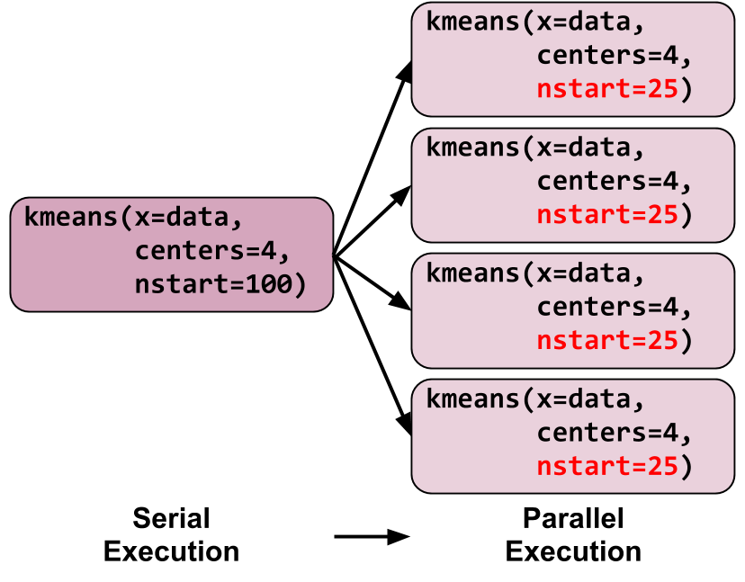
The operative procedure here is that we divided a single call of kmeans into four calls of kmeans:

Each of these four kmeans invocations only calculate a quarter of the original 100 starting points, and since starting points are all independent, we can now potentially run these four kmeans concurrently.

3.2. mclapply: shared-memory parallelism

Now that we have a parallelizable form of this simple k-means problem, actually parallelizing it is quite simple. There are literally two changes you have to make, highlighted in blue below:

library(parallel)

data <- read.csv('dataset.csv')

parallel.function <- function(i) {
    kmeans( data, centers=4, nstart=i )
}

results <- mclapply( c(25, 25, 25, 25), FUN=parallel.function )

temp.vector <- sapply( results, function(result) { result$tot.withinss } )
result <- results[[which.min(temp.vector)]]

print(result)

The parallel library, which comes with R as of version 2.14.0, provides the mclapply() function which is a drop-in replacement for lapply. The "mc" stands for "multicore," and as you might gather, this function distributes the lapply tasks across multiple CPU cores to be executed in parallel.

This is the first cut at parallelizing R scripts. Using shared memory (multicore) tends to be much simpler because all parallel tasks automatically share their R environments and can see the objects and variables we defined before the parallel region that is encapsulated by mclapply. All of the hard work is in restructuring your problem to use lapply when, serially, it wouldn't necessarily make sense.

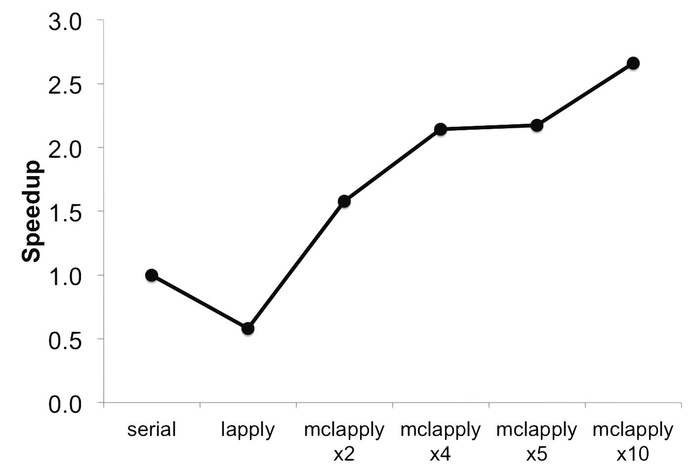
The performance isn't half bad either. By changing the MC_CORES environment variable, we can see how well this mclapply approach scales:

The downside is that this shared memory approach to parallelism in R is limited by how many cores your computer has. Modern supercomputers achieve parallelism via distributed memory, meaning many nodes (discrete computers in their own right) do not share memory and need to be explicitly given all of the variables and objects that were created outside of the parallel region.

3.3. parLapply: distributed-memory parallelism

To use more than one node's worth of CPU cores with lapply-style parallelism, you have to use some type of networking so that each node can communicate with each other and shuffle the relevant data around. As such, there's a bit more bookkeeping involved with using an distributed memory version of lapply, but fortunately, the actual logic of your application doesn't need to change much. Here is what a multi-node version of our parallel k-means would look like using parLapply instead of mclapply:

library(snow)

data <- read.csv( 'dataset.csv' )

parallel.function <- function(i) {
    ;kmeans( data, centers=4, nstart=i )
}

cl <- makeCluster( mpi.universe.size(), type="MPI" )
clusterExport(cl, c('data'))

results <- parLapply( cl, c(25,25,25,25), fun=parallel.function )

temp.vector <- sapply( results, function(result) { result$tot.withinss } )
result <- results[[which.min(temp.vector)]]
print(result)

stopCluster(cl)
mpi.exit()

Once again, differences are highlighted in blue. Notably,

1. We use the snow library instead of the parallel library. This is not strictly necessary, but as I'll discuss below, having snow installed allows you to use a few additional parallel backends.
2. We must create a "cluster" object using the makeCluster function. This "cluster" will be what determines what nodes and cores the parLapply function are available for work distribution.
3. Because we are using distributed memory, not all of our worker CPUs can see the data we have loaded into the main R script's memory. Thus, we need to explicitly distribute that data to our worker nodes using the clusterExport function.
4. To be completely proper, we need to tear down the cluster we built at the end of our script using stopCluster(cl). The mpi.exit() is required because we chose to use the MPI cluster type.

The "bookkeeping" required to set up and tear down clusters are the biggest difference between using shared-memory mclapply and this distributed-memory parLapply, but parLapply is actually a generalization of mclapply. This is a result of the fact that when creating clusters using the makeCluster function, you have the option to select different parallel backends that use shared memory or distributed memory:

3.3.1. MPI clusters

The type="MPI" uses MPI for its parallel operations, which is inherently capable of distributed memory. There are a few benefits:

• You can utilize any high-performance networking like InfiniBand if it is available on your parallel computing hardware
• You can also leverage MPI's integration with your resource manager so that you don't need to know the hostnames of all of your job's nodes

But there are also some complications:

• You need to install Rmpi, which can be unpleasantly difficult
• You need to launch your R script from within an MPI environment which is a little more complicated

If your parallel computing platform already has MPI installed and you can install Rmpi yourself (or have a handy staffmember who can help you), using type="MPI" is definitely the best way to use distributed-memory parallelism with parLapply simply because large parallel computers are designed to run MPI at their foundations. You might as well work with this as much as you can.

3.3.2. PSOCK clusters

The type="PSOCK" uses TCP sockets to transfer data between nodes.

The benefits:

• PSOCK is fully contained within the parallel library that ships with newer versions of R (> 2.14) and does not require external libraries like Rmpi
• It also runs over regular old networks (and even the Internet!) so you don't need special networking as long as your cluster hosts can communicate with each other

But there are also some complications:

• You are stuck using TCP which is relatively slow in terms of both bandwidth and latency
• You need to explicitly give the hostnames of all nodes that will participate in the parallel computation

Creating a PSOCK cluster is similar to launching an MPI cluster, but instead of simply saying how many parallel workers you want (e.g., with the call to mpi.universe.size() we used in the MPI cluster example above), you have to lay them all out, e.g.,

mynodes <- c( 'localhost', 'localhost', 'node1', 'node1', 'node2', 'node2' )
makeCluster( mynodes, type='PSOCK' )

In the above example, we indicate that we will want to use two parallel workers on the same machine from which this R script was launched (localhost appears twice) as well as two workers on a machine named node1 and two more on node2.

Ultimately, PSOCK works well in small-scale computing environments where there are a lot of loosely coupled computers available. For example, if your lab has a few workstations that aren't in use, you can use all of their idle CPUs to process a single R job using parLapply without having to configure any sort of complex parallel computing environment using PSOCK.

3.3.3. FORK clusters

Finally, type="FORK" behaves just like the mclapply function discussed in the previous section. Like mclapply, it can only use the cores available on a single computer, but it does not require that you clusterExport your data since all cores share the same memory. You may find it more convenient to use a FORK cluster with parLapply than mclapply if you anticipate using the same code across multicore and multinode systems.

foreach-based parallelism is another way of thinking about this sort of parallelism and is covered in the next section.