vector database

Vector databases store high-dimensional vectors (embeddings) in a way that makes searching for similar vectors (based on something like Euclidean distance) very quick.

For example, if the abstract for a paper is converted into a vector embedding, you could query a vector database for other vectors that are nearby in the embedding space. Each nearby vector in the database would tie back to an abstract that had similar semantic meaning, because the embedding model used to create all embeddings was trained to embed abstracts in a way that captures the essence of their meaning.

Put differently, vector databases let you do this:

1. Start with some text (or an image, or whatever else). It can be a query or it can be some reference data that might be useful for answering other queries.
2. Run that text through an embedding model. This converts it into an embedding (which is a vector) whose values represent where it lives in some high-dimensional space that represents the core meaning of that text. Other vectors with similar values, by virtue of the embedding model, have similar meanings.
3. Insert the embedding into a vector database.
4. Query the vector database with a new vector. The vector database returns other nearby vectors, their closeness, and pointers back to the original text that generated each returned vector. That original text can be PDF files in an object store or whatever.

Vector search

Brute-force search

Vectors in a vector database are literally multi-dimensional arrays of floating point values. The simplest way to find similar vectors is through brute-force distance calculation. If you have a query, the process is…

1. Generate the embedding for the query
2. For each vector in the vector database, calculate the distance between it and the query vector (step #1). This might be a simple Euclidean distance (i.e., using the Pythagorean theorem)
3. Sort the distances calculated in #2
4. Pick the top-k shortest distances. Those vectors are the nearest neighbors.

This is obviously extremely expensive, because the amount of vector comparisons that must be done scales linearly with the number of vectors in the database. If your database contains 1,000 vectors, every query has to perform 1,000 distance calculations. For this reason, vector databases never do this at scale.

Approximate nearest neighbor search

Vector databases typically use Approximate Nearest Neighbor (ANN) search, which trades perfect accuracy for speed. Instead of returning the top-k nearest vectors in the entire database, it returns the top-k vectors that are probably the nearest vectors which is good enough for semantic search applications.

Hierarchical Navigable Small World (HNSW)

HNSW¹ is a graph-based approach to building an index for a vector database:

1. Every vector in the database exists at layer 0 and is connected to its 16 nearest neighbors.
2. A random sample of vectors in layer 0 are also copied into layer 1. These layer-1 copies are then connected to 16 nearest layer-1 neighbors.
3. A random sample of vectors in layer 1 are also copied into layer 2. These layer-2 copies are then connected to 16 nearest layer-2 neighbors.
4. …and so on.

When a vector query comes in,

1. It starts at the highest layer (e.g., layer 4) and finds the nearest-neighbor vector to the input query’s vector. Let’s call that nearest neighbor Bob.
2. It then descends to the next layer down (layer 3) and searches only Bob’s 16 nearest neighbors for the one closest to the input query’s vector. Let’s call that neighbor Bob Jr.
3. It then descends to the next layer down (layer 2) and searchest only Bob Jr.’s 16 nearest neighbors for the closest one.
4. …and so on.

I picture the query process like this:

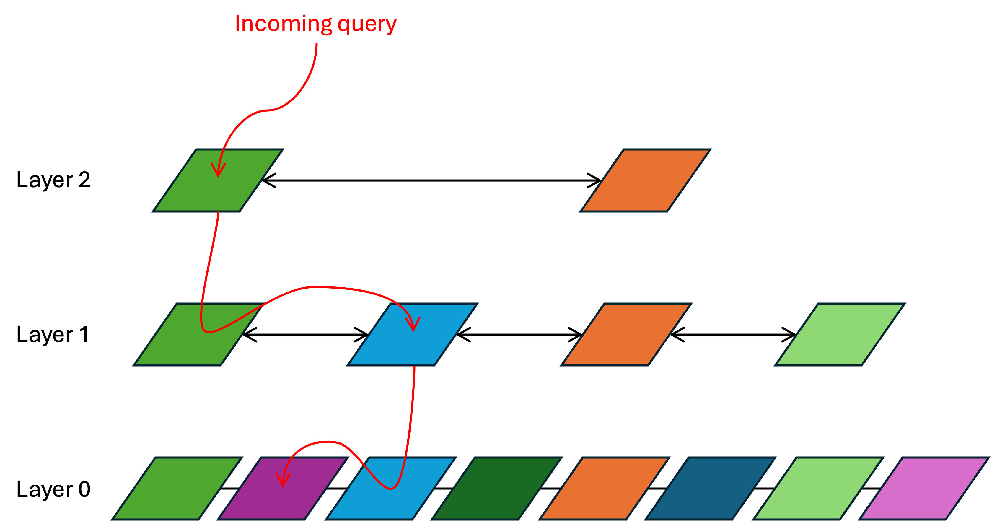
In the above, there are three layers and each vector has only two nearest neighbors:

• The incoming query lands at the topmost layer (layer 2). The distance between it and every layer-2 vector is calculated. This is brute-force, but layer 2 has so few vectors in it that this calculation is still very quick. The result is that the green vector is the nearest neighbor.
• Search then descends to layer 1 and looks at the nearest neighbors around that same green vector. It determines that, of the green vector and its nearest neighbors, the blue vector is the closest.
• Search then descends to layer 0 and looks at the nearest neighbors around the blue vector. It determines that, of the blue vector and its nearest neighbors, the purple vector is the closest. That is the approximate nearest neighbor to the incoming query.

This is ultimately a graph traversal, and it requires a lot of pointer chasing. As a result, these HNSW vector indices typically must fit in DRAM in order for them to be fast.

As of 2026, most vector databases use HNSW indices.

Hierarchical clustering

The VAST vector database uses hierarchical clustering instead of HNSW to build its vector indices.² It is constructed as follows:

1. Every vector in the vector database exists at layer 0, and k-means clustering is applied to group every vector into clusters of up to 1,000 vectors.
2. The centroid of every cluster at layer 0 is calculated. These centroids are then copied into layer 1. All layer 1 centroids are grouped into clusters of up to 1,000 layer-1 centroids.
3. The centroid of every layer-1 cluster is calculated and copied into layer 2. Layer-2 centroids are grouped into clusters of up to 1,000 layer-2 centroids.
4. … and so on.

A key advantage of hierarchical clustering over HNSW is that the promotion of vectors into higher layers is not random; it is locality-aware. This means that every time the search descends one layer lower in the index, it is zeroing in on a localized area within the vector search. This reduces the breadth of the pointer chasing and eliminates the need to scan widely across the vector space at each layer.

Comparing HNSW and clustering

HNSW effectively trades storage locality for graph navigability. Inserts are fast because no attempt is made to store similar vectors physically close to each other. As a result, search requires unpredictable, pointer-chasing I/O that effectively requires storing the entire HNSW graph in DRAM.

Hierarchical clustering makes the opposite tradeoff. Inserts are slower because new vectors are placed into the correct cluster as a part of the insertion. However, clusters can be mapped to physical hardware in whatever way is optimal for performance, allowing queries to be pre-optimized. In practice, clusters can be placed on hardware in a way that avoids the wide pointer chasing required by HNSW indices.

Examples

Name	Architecture	QPS	Vector count
Milvus	scale-out	”tens of thousands"	"billions”
Chroma	embedded to scale-out

Chroma deploys compute on top of someone else’s object store for persistence, so its performance is limited by the latency of the underlying storage.

Theoretical limits

DeepMind established a fundamental limit to how large a vector database can be before it stops returning useful results.³ A few notes:

• This study holds true regardless of if one uses exact nearest neighbors or ANNs.
• There is a limit to how much dot-product similarity can express.
• Increasing vector length increases the expressivity of the vector space, but every vector length has a fundamental limit.
• Queries with predicate logic (must / must not / and / but not) fare worse; vector similarity cannot accurately find similarity above a certain complexity in these cases.

The solution to this limit is to be more sophisticated in how you determine similarity. For example,

• employ hybrid filtering or predicate filtering alongside similarity
• use reranking that actually reads chunks after the first similarity search to carefully evaluate relevance
• use multiple vector spaces to represent each chunk

Footnotes

1. Efficient and Robust Approximate Nearest Neighbor Search Using Hierarchical Navigable Small World Graphs | IEEE Transactions on Pattern Analysis and Machine Intelligence ↩

2. The Architecture Behind Our 11× Vector Benchmark - VAST Data ↩

3. [2508.21038] On the Theoretical Limitations of Embedding-Based Retrieval ↩